Feature Story

Ray Tracing for Beginners

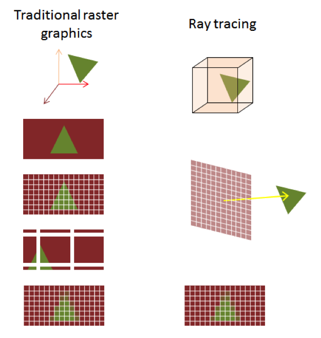
For the past three decades, there have been two main schools of thought dominating the center stage of 3D graphics: rasterization and ray tracing.

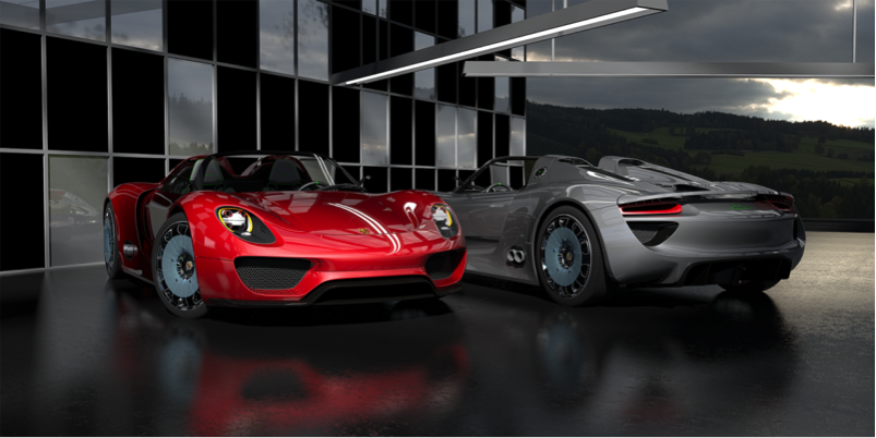
If you really don't care about the finer details and you want a five-second explanation of ray tracing, then all you need to know is that ray tracing will turn something like this:

into this:

Since the 1990s, we have seen an exponential increase in rasterized GPU performance. However, each advance in visual quality has made content generation more complicated and costly. Every single effect (each shadow, reflection, highlight, or subtle change in illumination) must be anticipated by the designer or game engine, and special-cased.

This work often results in massive game title budgets, slower time to market, and ultimately less content on the platform.

Ray tracing takes a different approach to rasterized rendering by closely modeling the physics of light; it provides the only way to achieve photorealism for interactive content at an affordable price. Even though you might not have heard of ray tracing before, there's a high probability you've already seen what it can do: ray tracing is the primary technique used for special effects rendering in movies. In addition, the techniques to produce realistic-looking games also use ray tracing offline in a process called pre-baking.

Finally, ray tracing has been used to seamlessly blend captured real life with computer-generated images (i.e. VR/AR applications) as it is much better at simulating optical effects like reflection and refraction, scattering, and dispersion phenomena compared to traditional rendering methods like scanline.

The main reason why ray tracing hasn't been fully embraced at a larger scale is that traditionally any real-time ray tracing application needed a GPU beast running an OpenCL-based algorithm to produce images similar to the one above. Since most people don't have a water-cooled rig of 300W GPUs lying around their living room, ray tracing never really took off in a big way. The problem with using GPU compute for ray tracing is its inefficiency in handling the complex issue of keeping track of coherency between rays. You see, GPU compute is extremely good at data parallel operations that obey a certain (and predictable) structure. Image processing is a perfect application for GPU compute: you apply the same filter over and over again on every pixel in a rinse and repeat fashion.

Imagination's PowerVR Wizard, for example, abandons this flawed computation-intensive approach and implements a much better solution that is modeled after how ray tracing actually works.

PowerVR Ray Tracing GPUs start with a pixel. For each step, the engine tracks intersections of a ray with a set of relevant primitives of the scene and performs geometry processing using a shader, exactly as in rasterization. Behind the scenes, the RTU (ray tracing unit) assembles the triangles into a searchable database representing the 3D world.

When a shader is run for each pixel, rays are cast into the 3D world. This is when the RTU steps in again to search the database to determine which triangle is the closest intersection with the ray. If a ray intersects a triangle, the shader can contribute color into the pixel, or cast additional rays; these secondary rays can in turn cause the execution of additional shaders.

All of this wizardry (pardon the pun) is implemented directly in hardware which makes the whole GPU very fast at handling specialized ray tracing tasks and conserves a lot of power, making it 100x more energy efficient than competing solutions.

This is the vital and main advantage of using an RTU alongside a traditional GPU for ray tracing. By using specialized hardware to keep track of secondary rays and their coherency, an impressive speedup of the complicated computational process is achieved – this results in a higher degree of visual realism provided in real time.

Implementing fast, ray traced soft shadows in a game engine

Not only does ray tracing create more accurate shadows that are free from the artifacts of shadow maps, but ray traced shadows are also up to twice as efficient; they can be generated at comparable or better quality in half the GPU cycles and with half the memory traffic (more on that later).

So let's take you through the process of implementing an efficient technique for soft shadows.

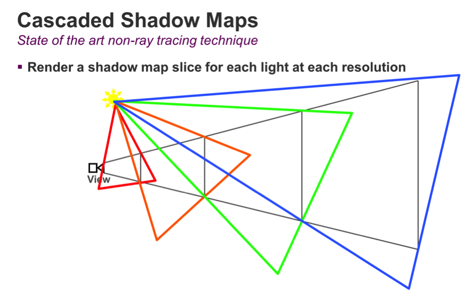
Cascaded shadow maps in traditional rasterized graphics

Firstly, let's review cascaded shadow maps – the state of the art technique used today to generate shadows for rasterized graphics. The idea behind cascaded shadow maps is to take the view frustum, divide it up in a number of regions based on distance from the viewpoint, and render a shadow map for each region. This will offer variable resolution for shadow maps: the objects that are closer to the camera will get higher resolution, while the objects that fall off into the distance will get lower resolution per unit area.

In the diagram below, we can see an example of several objects in a scene. Each shadow map is rendered, one after another, and each covers an increasingly larger portion of the scene. Since all of the shadow maps have the same resolution, the density of shadow map pixels goes down as we move away from the viewpoint.

Finally, when rendering the objects again in the final scene using the camera's perspective, we select the appropriate shadow maps based on each object's distance from the viewpoint, and interpolate between those shadow maps to determine if the final pixel is lit or in shadow.

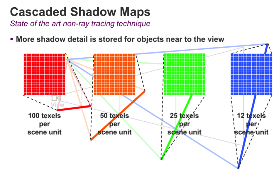
All of this complexity serves one purpose: to reduce the occurrence of resolution artifacts caused by a shadow map being too coarse. This works because an object further away from the viewpoint will occupy less space on the screen and therefore less shadow detail is needed. And it works nicely – although the cost in GPU cycles and memory traffic is significant.

Enter ray traced shadows

Ray traced shadows fundamentally operate in screen space. For that reason, there is no need to align a shadow map's resolution to the screen resolution; the resolution problem just doesn't exist.

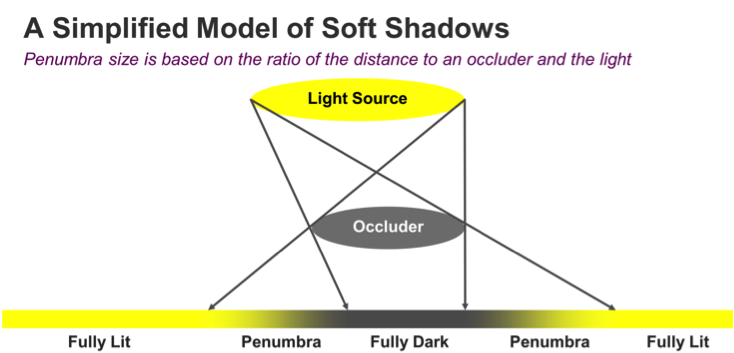
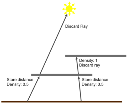
The basic ray traced shadow algorithm works like this: for every point on a visible surface, we shoot one ray directly toward the light. If the ray reaches the light, then that surface is lit and we use a traditional lighting routine. If the ray hits anything before it reaches the light, then that ray is discarded because that surface is in shadow. This technique produces crisp, hard shadows like the ones we might see on a perfectly cloudless day.

However, most shadows in the real world have a gradual transition between lighter and darker areas – this soft edge is called a penumbra. Penumbras are caused by different factors related to the physics of light; even though most games model light sources as a dimensionless point source, in reality light sources have a surface. This surface area is what causes the shadow softness. Within the penumbra region, part of the light is blocked by an occluding object, but the remaining light has a clear path. This is the reason you see areas that are not fully in light and not fully in shadow either.

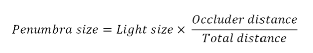
The diagram below shows how we can calculate the size of a penumbra based on three variables: the size of the light source (R), the distance to the light source (L), and the distance between the occluder and the surface on which the shadow is cast (O). By moving the occluder closer to the surface, the penumbra is going to shrink.

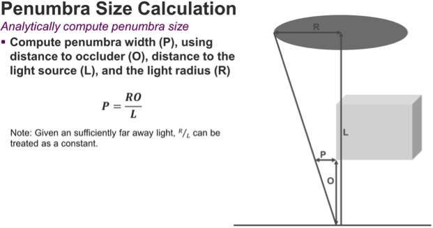
Based on these variables, we derive a simple formula for calculating the size of the penumbra.

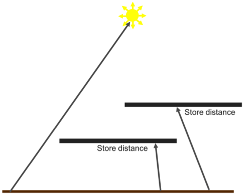
Using this straightforward relationship, we can formulate an algorithm to render accurate soft shadows using only one ray per pixel. We start with the hard shadows algorithm above; but when a ray intersects an object, we record the distance from the surface to that object in a screen-space buffer.

This algorithm can be extended to support semi-transparent surfaces. For example, when we intersect a surface, we can also record whether it is transparent; if the surface is transparent, we choose to continue the ray through the surface, noting its alpha value in a separate density buffer.

This method has several advantages over cascaded shadow maps or other common techniques:

There are no shadow map resolution issues since it is all based in screen space
There are no banding, noise or buzzing effects due to sampling errors
There are no biasing problems (sometimes called Peter-Panning) since you are shooting rays directly off geometry and therefore getting perfect contact between the shadow and the casting object

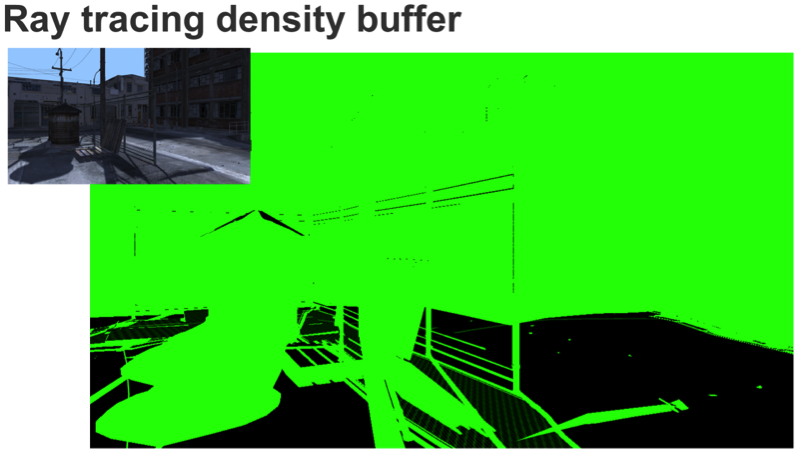
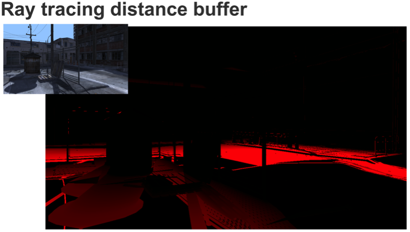
Below we show an example of the buffers that are generated by the ray tracing pass (we've uploaded the original frame here).

First, we have the ray tracing density buffer. Most of the objects in the scene are opaque, therefore we have a shadow density of 1. However, the fence region contains multiple pixels that have values between 0 and 1.

Next up is the distance to occluder buffer. As we get further away from the occluding objects, the value of the red component increases, representing a greater distance between the shadow pixel and the occluder.

Finally we run a filter pass to calculate the shadow value for each pixel using these two buffers.

Firstly, we work out the size of the penumbra affecting each pixel, use that penumbra to choose a blur kernel radius, and then blur the screen-space shadow density buffer accordingly. For a pixel that has a populated value in the distance to occluder buffer, calculating the penumbra is easy. Since we have the distance to the occluder, we just need to project that value from world space into screen space, and use the projected penumbra to select a blur kernel radius.

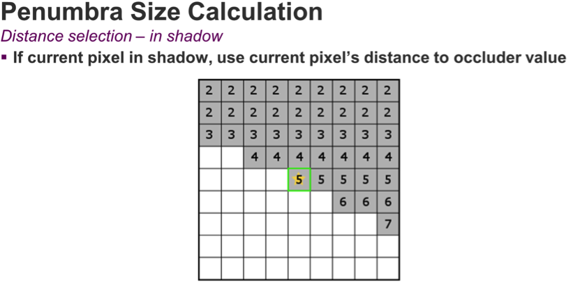
When the pixel is lit, we need to work a little harder. We use a cross search algorithm to locate another pixel with a ray that contributes to the penumbra. If we find any pixels on the X or Y axis that are in shadow (i.e. have valid distance values), we'll pick the maximum distance to occluder value and use it to calculate the penumbra region for this pixel; we then adjust for the distance of the located pixel and calculate the penumbra side.

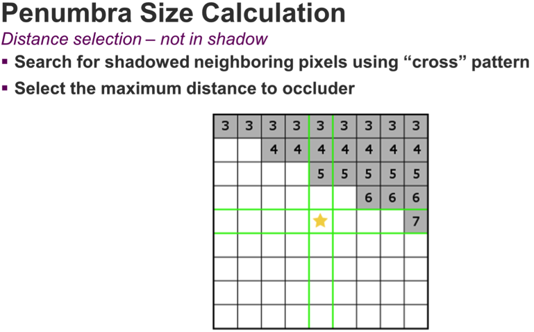
From here on, the algorithm is the same: we take the size of the penumbra from world space and project it into screen space, then we figure out the region of pixels that penumbra covers, and finally perform a blur. In the case where no shadowed pixel is found, we assume our pixel is fully lit.

Below we have a diagram representing our final filter kernel.

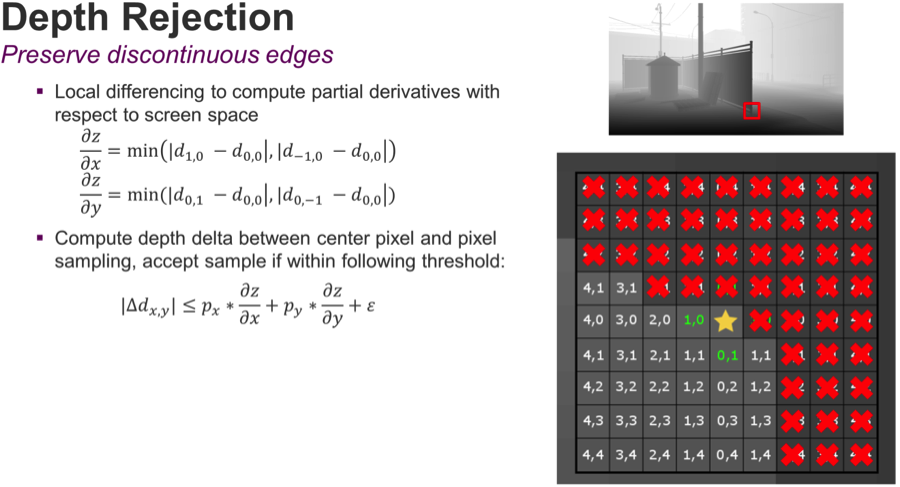
We are covering the penumbra region with a box filter and sample it while still being aware of discontinuous surfaces. This is where depth rejection comes to our aid; to calculate the depth rejection values, we use a local differencing to figure out the delta between the current pixel and certain values on the X and Y axis. The result will tell us how far we need to step back as we travel in screen space. As we're sampling our kernel, we'll expand the depth threshold based on how far away we are from the center pixel.

In the example above, we have rejected all the samples marked in red because the corresponding area belongs to the fence and we are interested in sampling a spot on the ground. After the blurring pass, the resulting buffer represents an accurate estimate of the shadow density across the screen.

Complete results: cascaded shadow maps vs. ray traced shadows

The images below compare an implementation of four slice cascaded shadow maps at 2K resolution versus ray traced shadows. In the ray traced case, we retain the shadow definition and accuracy where the distance between the shadow casting object and the shadow receiver is small; by contrast, cascaded shadow maps often overblur, ruining shadow detail.

Clicking on the full resolution images reveals the severe loss of image quality that occurs in cascaded shadow maps.

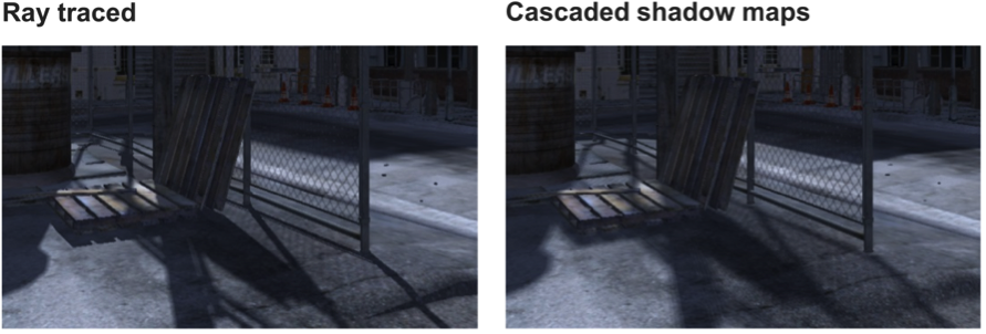
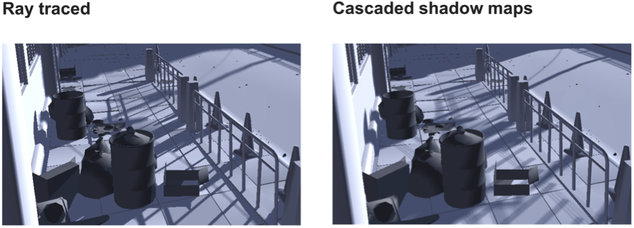
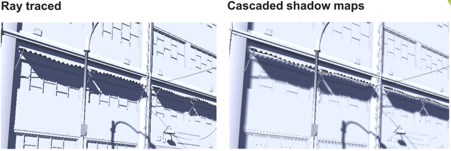
In the second and third examples, we've removed the textures so we can highlight the shadowing.

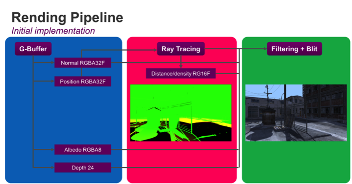
Optimizing the ray tracing algorithms

The diagram below describes the initial implementation of the ray tracing hybrid model described in this article.

The first optimization we can make is to cast fewer rays. We can use the information provided by dot (N, L) to establish if a surface is back facing a ray. If the dot (N, L) result is less or equal to 0, we don't need to cast any rays because we can assume the pixel is shadowed by virtue of facing away from the light.

Looking at the rendering pipeline, there are further optimizations we can make. The diagram below shows the standard deferred rendering approach; this approach involves many read and write operations and costs bandwidth (and therefore power).

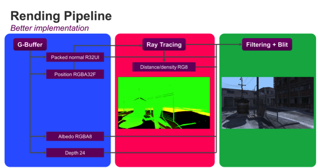
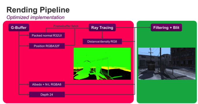
The first optimization we've made is to reduce the amount of data in each buffer by using data types that don't have any more bits than the bare minimum needed; for example, we can pack our distance density buffer into only 8 bits by normalizing the distance value between 0 and 1 since it doesn't require very high precision. The next step is to collapse passes; if we use the framebuffer fetch extension, we can collapse the ray tracing and G-Buffer into one pass, saving all of the bandwidth of reading the G-Buffer from the ray emission pass.

Memory bandwidth usage analysis

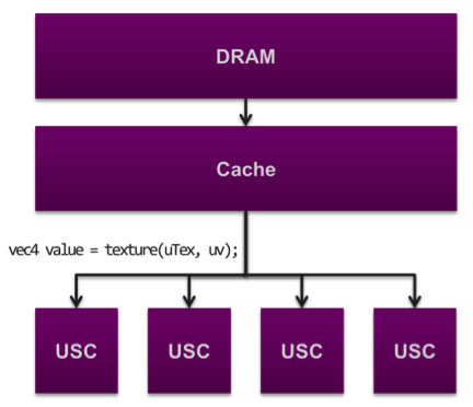
Before we look at the final numbers, let's spend some time looking at memory traffic. Bandwidth is the amount of data that is accessed from external memory; memory traffic consumes bandwidth. Every time a developer codes a texture fetch, the shading cluster (USC) in a PowerVR Rogue GPU will look for it inside the cache memory; if the texture is not stored locally in cache, the USC will access DRAM memory to get the value. For every access to external memory, the chip will incur significant latency and the device will consume more power. When optimizing a mobile application, the goal of a developer is to always minimize the accesses to memory.

By using specialized instruments to look at bandwidth usage, we can compare cascaded shadow maps with ray traced soft shadows on a PowerVR Wizard GPU. In total, the cascaded shadow maps implementation consumes about 233 MB of memory while the same scene rendered with ray traced soft shadows requires only 164 MB. For ray tracing, there is an initial one-time setup cost of 61 MB due to the acceleration structure that must be built for the scene.

This structure can be reused from frame to frame, so it isn't part of the totals for a single frame. We've also measured the G-Buffer independently to see how much of our total cost results from this pass.

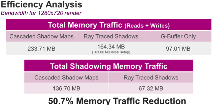
Therefore, by subtracting the G-Buffer value from the total memory traffic value, shadowing using cascaded maps requires 136 MB while ray tracing is only 67 MB, a 50% reduction in memory traffic.

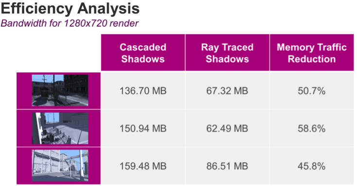
We notice similar effects in other views of the scene depending on how many rays we are able to reject, how much filtering we have to perform. Overall, we get an average of 50% reduction in memory traffic using ray traced shadows.

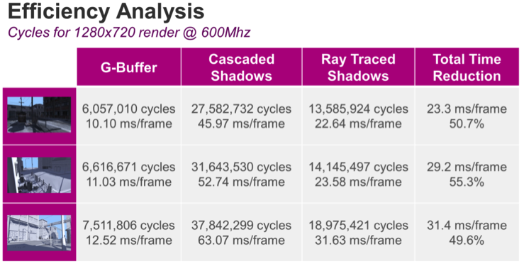
Looking at total cycle counts, the picture is even better; we see an impressive speed boost from the ray traced shadows. Because the different rendering passes are pipelined in both apps (i.e. the ray traced shadows app and the cascaded shadow maps app) we are unable to separate how many clocks are used for which pass. This is because portions of the GPU are busy executing work for multiple passes at the same time. However, the switch to ray traced shadows resulted in a doubling of the performance for the entire frame!

Even though rasterized content today already looks pretty impressive, there are still big challenges to close the gap between the photorealism that ray tracing offers and what we see on current-generation mobile and desktop devices.

Alexandru Voica is senior technology marketing specialist at Imagination Technologies. Imagination is a global technology leader whose products touch the lives of billions of people across the globe. The company's broad range of silicon IP (intellectual property) includes the key processing blocks needed to create the SoCs (Systems on Chips) that power mobile, consumer and embedded electronics.

Return to: 2015 Feature Stories